
Review
A previous post discussed how the decision tree algorithm classifies items using the gini impurity index–a simple score that is easily calculated. Please visit this post for some background information or a refresher if necessary.
Pitfalls of Decision Trees
Decision trees are relatively straightforward, regardless whether it is built on the gini impurity index or entropy gain (well-explained here). On a fundamental level, decision trees classify items basically on how similar their attributes are to items in a certain class.
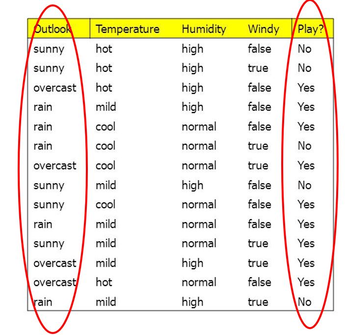
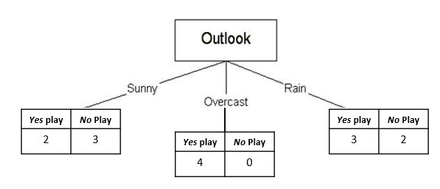
Using the same example from the previous post about deciding whether or not one plays outside, a decision tree created from this data will always declare that, assuming an overcast outlook, playing outside is the correct course of action regardless of temperature, humidity, and windiness.

Intuitively, this will not always be true. This is because the dataset is obviously too small, so the algorithm wouldn’t be able to learn new patterns. However, it also represents an inherent weakness in using decision trees; they are often inflexible and inaccurate, especially when new data does not follow similar trends is introduced. Ie. every instance where one does not go outside during an overcast would be misclassified with the above decision tree. Hence, the decision tree has been overfitted to the data.
Democracy in an Algorithm
This is exactly what the Random Forest algorithm makes up for. As the name suggests, rather than having a single tree determine every classification, the algorithm “plants” many trees that run the classification, and they collectively “vote” on the best classification.

However, this only works if every tree is different from each other, but how can this be if each tree relies on the same dataset? After all, a tree grown on the same dataset (assuming similar parameters) will have the same root, internal, and leaf nodes.
The solution involves bootstrapping, which is a sampling with replacement method (explained here) used to create new datasets. To briefly explain, this means that random rows are selected from the original dataset with replacement (Ie. the same row can be selected more than once) to create a new dataset:

The new subset has the same number of samples (rows) as the original dataset, but is obviously different since not all rows were sampled. Therefore, the decision tree created from this subset of data would have different nodes and possibly a different classification overall!
This sampling can be repeated to create a plethora of different trees that, while mostly distinct, still retain the trends of the data since general patterns will more likely be sampled. This repeated bootstrapping can be aggregated to provide a general picture of the original dataset; this is also known as bagging (boostrapping + aggregating) In addition, it also allows the classification to be less rigid because different trees may cast different “votes.”
Evaluating Effectiveness
How does one assess if the Random Forest algorithm planted the “right” trees, so to speak? One method is through an out-of-bag sample. Typically, about 1/3 of the original data will not be used (If you want to know why, click here). Therefore, the data that does not end up being used to make decision trees in the forest can instead be used to test it.
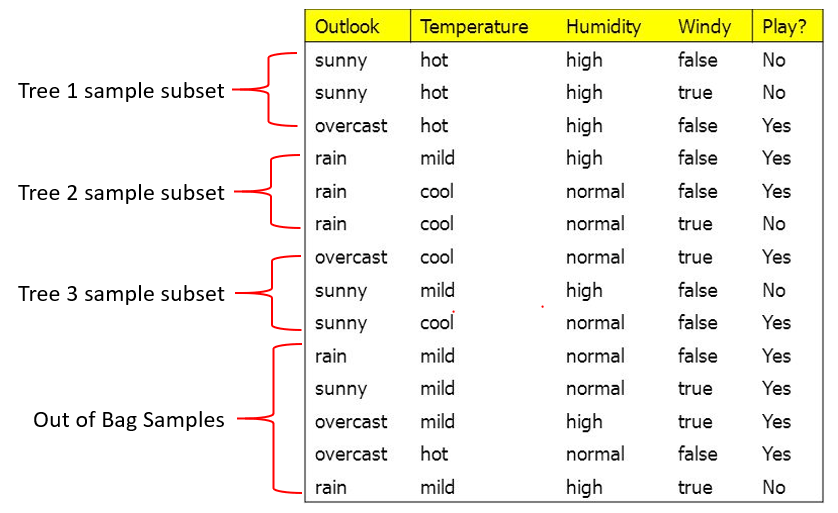
In the above scenario, there are 5 out-of-bag samples (abbreviated OoBs) that can be used to test the effectiveness of the forest. Consider the first sample:

The parameters of a rainy outlook, mild temperatures, normal humidity, and lack of wind can be placed through each of the trees. Let’s assume that each tree voted, and these were the results:
| Tree 1 Vote | Yes Play |
| Tree 2 Vote | Yes Play |
| Tree 3 Vote | No Play |
| Overall Classification | Yes Play |
This would be the correct classification. This is then repeated for every OoB sample to see how well the forest does. In the end, the total accuracy of the forest can be determined by dividing the number of correct classifications by the total number of OoB samples, thus giving us a relative idea of how well the Random Forest did and allows us to tweak parameters as needed.
Overall, Random Forest is a very versatile classification algorithm that avoids overfitting on training data like decision trees. Its usage of either validation or OoB error allows two ways to measure the algorithm’s performance, even when there may not be so much data. Lastly, Random Forest can even deal with missing data, but that will be covered in a separate article, since there’s a bit more math to it.
