A Mathless Breakdown of Decisions Trees and the Gini Impurity Index

The decision tree algorithm is one of the first learned by most aspiring data scientists because while the underlying math may be tedious, the overall logic is pretty simple to understand, at least on a surface level. At its core, a decision tree is a classifier algorithm, which means it has to make a decision about what group something falls into based on the attributes of that thing:

An oversimplified, but intuitively harsh decision tree

So in this case, this decision tree has decided that anyone over the age of 29 must exercise in the morning to be fit, which I sincerely hope is not the case, but that’s a topic for another time. The structure of the above example is also more commonly represented like this:

To put things in layman’s terms:

• Root Node – only has arrows point away from it to either an internal node or a leaf node (Age<30)
• Internal Node(s)- Has both arrows pointing to it and arrows pointing away from it (Eats lots of pizza & exercises in the morning)
• Leaf Node(s)- Only has arrows pointing to it (Fit & Unfit)

It is generally easy to determine what should be the leaf node; often, it is a binary classification where something is either true or false. However, the same cannot be said root and internal nodes. Suppose in our example, the root node (Age<30) is switched with the internal node (exercises in the morning) like so:

This intuitively makes less sense to us as certain routes through the tree are illogical. For example, the above tree basically guarantees that anyone below the age of 30 is fit even if they don’t exercise in the morning. Therefore, the placement of different categories at the correct nodes are critical in having a tree that makes the most sense.

This may because obvious in some cases like the above scenario, but certain other classifications are much harder to determine such as which factors should be the root node for determining heart disease. Furthermore, computers do not possess intuition and  fundamentally rely on numeric justification for how they construct trees. Understanding the numbers behind classification allow data scientists to effectively vet the algorithm and avoid pitfalls.

Let’s take a look at the one of the most used case studies for decision tree–deciding whether or not you should go play outside based on the weather:

The above chart shows when you’ve decided to go outside to play and each instance’s weather factors. For now, let’s just focus on the outlook and play column. The decisions to play or not is understandably the leaf node, since that is the final classification (Ie. decision) we’d like to make. However, deciding which of the four columns should be the root node isn’t as straightforward as our previous example of being fit or unfit. Inherently, we’d like the column that affects the “play” decision the most to be the root node, but how can we empirically justify that one column affects that result more than other columns. Enter the gini impurity index.

The scary-looking formula above might be what first pops up if you Googled gini impurity index, but the mathematical notation simply looks complicated. This is the gini impurity index stated a different way:

Gini  = 1 – (probability of yes)² – (probability of no)^{2  *}

Let’s apply this back to figure 1 and calculate the gini impurity of outlook as the internal node. In this case, there are 3 different types of outlook — sunny, overcast, and rainy.  Each of those scenario may have some effect on whether or not we play outside:

To calculate the probability yes or no for each outlook, we use the following:

Probability of yes= (# of yes) / (total # of cases)

Probability of no= (# of no) / (total # of cases)

Therefore gini impurity for each outlook is can be defined like this:

Gini of Outlook Type = 1 – (# yes/total)² – (#no/total)²

Gini Sunny = 1 - (2/5)2 - (3/5)2 =.48 
Gini Overcast = 1 - (4/4)2 - (0/4)2 = 0
Gini Rainy = 1 - (3/5)2 - (2/5)2 =.48 

The gini index is a number we want to be minimize down to zero, if possible. To reiterate, this number is a way of quantifying the effect of one factor on your decision to play or not. A gini of 0, like with overcast, indicates that you will always go outside and play when the outlook is overcast. This may not necessarily be true, but that is what the current data suggests.

Yet, the original question still stands, how do we know if the outlook column is the best root node? There is only last step–averaging the weighted gini indexes for each type:

Gini of Outlook Internal Node =

 (# of cases in sunny/total # of cases)*gini sunny
+
 (# of cases in overcast/total # of cases)* gini overcast+
 (# of cases in rainy/total # of cases)*gini rainy

This gives us the following:

Gini of Outlook Internal Node =

(5/14)*.48 + (4/14)*0 + (5/14)*.48 = .342

Finally, we have our answer! The gini weighted gini index of outlook as a root node is .342, but so what? How do we know that this should be the root node? Well, it’s relatively straightforward. We repeat the process to find the weighted gini index of a different column, which might make you feel a certain way…

But to speed things up, you can just follow along as we find the weighted gini index of the humidity column:

Then we can create a chart and determine the leaf node for both types of humidity:

Again, we calculate the gini impurity of both types of humidity:

Gini High humidity = 1 - (3/7)2 - (4/7)2  = .49
Gini Normal humidity = 1  - (6/7)2 - (1/7)2  = .24

And then finally calculate the weighted average of the entire column as a root node:

Gini of Humidity as Internal Node = (7/14)*.49 + (7/14)*.24 = .365

Critically, this is higher than if we had outlook as our root node, so we reject humidity as a root node. The algorithm then repeats the process again for both temperature and windiness and establishes the column with the lowest weighted gini impurity index as the root node, which would be the outlook column.

Those familiar with this problem will note that the tree looks something like this now:

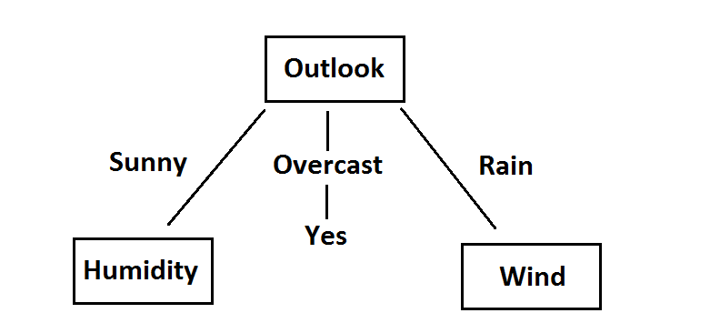
While it makes sense that overcast always leads to you going outside, how does the algorithm know to have a sunny outlook paired with humidity and rain paired with windiness? Again, it’s a matter of recalculating the gini impurity index, except that this time, we are determining the best internal node. Let’s focus on the sunny outlook along with humidity as our assumed internal node:

Humidity can be high or normal, so we perform two gini impurity calculations. Again, the leaf node is still the decision to play outside or not:

Gini High Humidity = 1 - (0/3)2 - (3/3)2  = 0
Gini Normal Humidity = 1 - (2/2)2 - (0/2)2  = 0

Thus, the weighted gini of humidity as an internal node for the sunny outlook is 0, which means that it would be the best internal node. For curiosity’s sake, we can also calculate the gini index if we instead use the windy column as an internal node:

Again, we’re only focused on the windy and play columns to calculate the gini index:

Gini Windy True = 1 - (1/2)2 - (1/2)2 = 0.5
Gini Windy False = 1 - (2/3)2 - (1/3)2 = 0.44

The weighted gini for windy as an internal node after sunny obviously would not be 0, so humidity is the internal node after a sunny outlook.  Since an overcast always leads to playing outside, windiness must be placed as the internal node after a rainy outlook.  The same process can be repeated for the next level and so on. Hence, the final tree looks like this.

The gini impurity index is one of two major ways of how the algorithm constructs the tree and ultimately classifies a decision. Though the math for the second method, entropy, might be slightly different, the idea behind it is relatively same–find the factors that most likely affects the overall outcomes, rank them, and construct a tree. Real-world data may not be so simple and succinct, but luckily this is where a computer’s ability to calculate gini impurity indices at lightning speed comes in handy.

Hopefully, this brief introduction into how a decision tree classifier functions shows you that while people love to throw around the word algorithm a lot in the data world, understanding them isn’t so bad; it just takes a bit of time and patience.