Hypothesis Testing with the Northwind Database

 

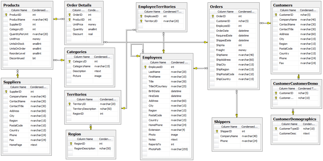
Microsoft’s Northwind Database has undoubtedly helped many aspiring individuals like myself in being able to play with data techniques such as querying data and building models from the database. There’s a lot that could be done with the database since its schema is relatively simple (see below):

 

Looking at the available information, there’s a lot that could be asked and answered using the database, but I chose four specific questions to pursue:

1. Do discounts have an effect on the number of items that consumers purchase? If so, what level of discount?
2. Do specific employees influence how many items are sold per transaction? If so, which employee does best?
3. Do customers prefer specific categories of items more so than others? If so, which category is most preferred?
4. Do different shipping companies have significantly different discrepancies between their order date and ship date? If so, which company seems to ship the fastest?

Although there were four questions, the basic structure for answering each question would essentially be the same:

1. Query required data via SQLite3 & perform the necessary -join’s and integrating the data into a pandas dataframe
2. Scrub the dataframe’s missing values
3. Establish null and alternative hypothesis
4. Conduct statistical test(s) to determine significance & effect size.
5. Summarize findings and readdress original inquiry

The first step of querying the data using SQL could be done with the panda library’s read_sql_query function. The important part is making an engine and binding it to a Session object and inserting it as a parameter every time you use the query (example below):

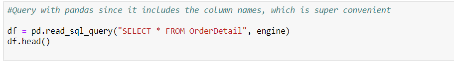
*As mentioned, there’s the added convenience of keeping column names!

However, there were two issues when I initially tried to query data for the first question. The first was that none of the tables that I was trying to call seemed to exist! I felt baffled until I decided to use the inspect function to get the names of the tables.

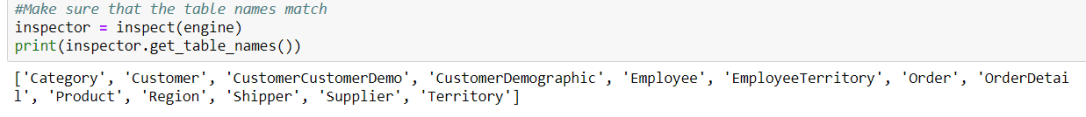
Ahh yes, the classic “schema switcheroo”

All the table names were the singular version of the names in the schema. Mystery number one solved. The second issue lacked an easy fix, though. Upon closer examination, I noticed that two things could represent how many items customers ordered—UnitsOnOrder and Quantity

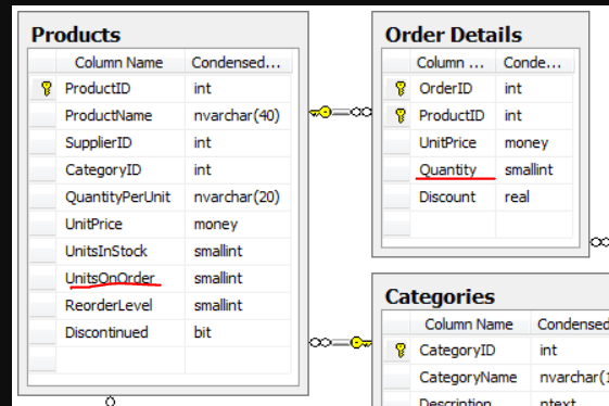
A quick google search did not reveal the answer as to which one would be my target variable, so I decided to use both of them to see how results would turn out. Perhaps I would know then.

I joined Order Details and Products using ProductID and excluded discontinued items from the dataframe and selected the product name, quantity, UnitsOnOrder, and discount. After briefly scanning for null values, the next step would be determining the null and alternative hypothesis¹ along with control and experimental groups. The null hypothesis would be that discounts make no difference in affecting consumer behaviors, while the alternative hypothesis would suggest the opposite—discounts can swing consumer patterns one way or the other. Thus, this necessitated a two-tailed test.

The control group in this case was straightforward since it aligned directly with the null hypothesis. Every other discount group will be the experimental group. Because it is the average amount of items bought by consumers that is being measured, a two-sample t-test would be the simplest approach. Before doing so, I needed to see how many discount groups I was working with:

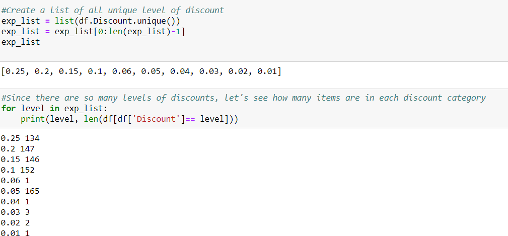
The third issue was obvious—a sheer lack of sample size for half of the discount levels. Since they made up such a small part of the over population, dropping them altogether would not pose an issue and would simplify the discount levels to increments of 5%.

I ran a two-tailed student t-test with every discount group acting individually as the experimental group against the control. I also looped this for both Quantity and UnitsOnOrder, and fortunately, that was enough to indicate what my target variable should be:

None of the results for UnitsOnOrder was significant, so it was dropped altogether. Instead, the p-values from the t-test comparisons with quantity had an interesting trend in that a discount of .1 (or 10%) was not statistically significant. In fact, the most significant result seemed to be the 15% discount, which runs a bit counterintuitive to economics. With the t-test, every category except the 10% discount group allowed for a rejection of the null hypothesis. Overall, it is possible to say that discounts do have a significant impact.

One of the weaknesses of a student t-test is that it can only test between two groups—a control and an experimental. To see if there is a proper effect of all groups on the target variable, ANOVA would be the best choice. Unfortunately, doing so raised some minor errors. The first was that each discount level was basically a category, which meant that it needed to be dummy-fied (yes, I’ll take credit for coining that). Second, the column names of each category returned a patsy error

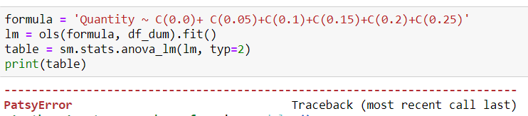
This meant having to endure the onerous task of renaming all the columns before running ANOVA again.

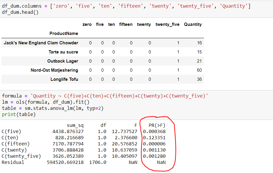
ANOVA supported the finding of the t-tests. However, I still needed to rationalize why the 15% discount group had the greatest impact on the amount of items sold. The most likely explanation, as usual, is that there are some other extraneous factors that can assist in explaining this trend. For example, it wouldn’t be hard to imagine that significantly discounted items were closer to the end of their shelf life, which would explain why the 25% category did have the biggest impact. As for 10%, maybe certain categories of items were often discounted at that amount at the end of their shelf life and these categories were undesirable near expiry date (e.g.milk). Being able to decipher and explain any deviation from what is expected is a critical skill because it allows for further investigations to be conducted and more questions to both arise and be answered.

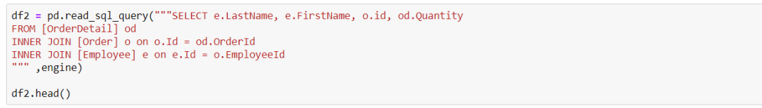
For all other questions after the first, the steps were relatively the same and much of the code could easily be copied and pasted to save time. In fact, there were only two steps that differed from question #1 across the other sections. The first obviously had to do with how to query the data since the desired information changed with each question, so it became necessary to look and query from different tables:

Question 2

Question 3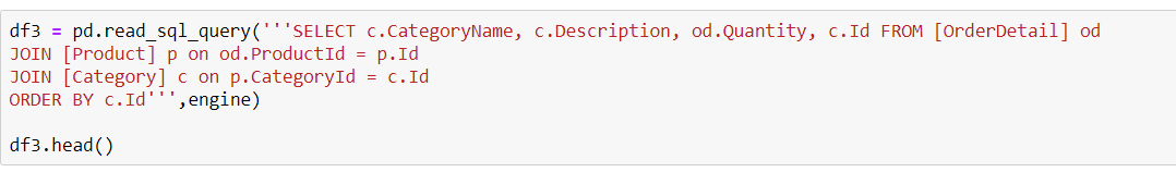

Question 4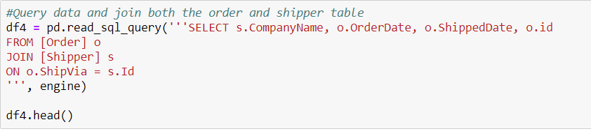

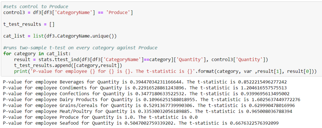
Unlike question #1, the other questions had no clear control group. Rather, one had to be arbitrarily chosen as the control group. Yet, this meant that any t-test conducted would simply measure a difference in means between the selected experimental group and that specific control group. To mitigate this, I ran t-tests twice. The first time, I randomly chose a control group and used the group with the lowest t-score as my new control group. That way, the second round of t-test can pick up on any significant differences.

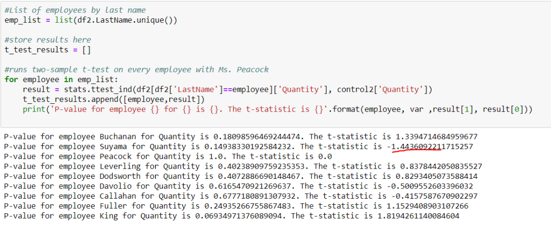
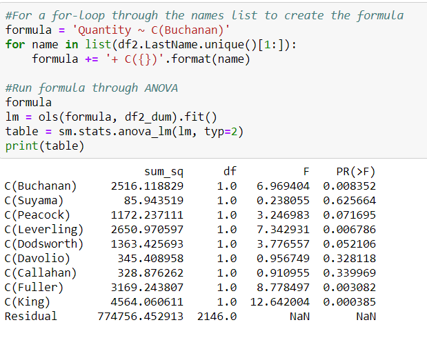
In the example above for question 2, I randomly chose Ms. Peacock to be my control group initially. This led to no p-value that met the .05 threshold, which meant that no employee performed significantly different compared to Ms. Peacock on sales quantity.  But then I switched the control group to Suyama, since he had the lowest t-score, which would indicate that his average quantity would be at the lowest end of the spectrum

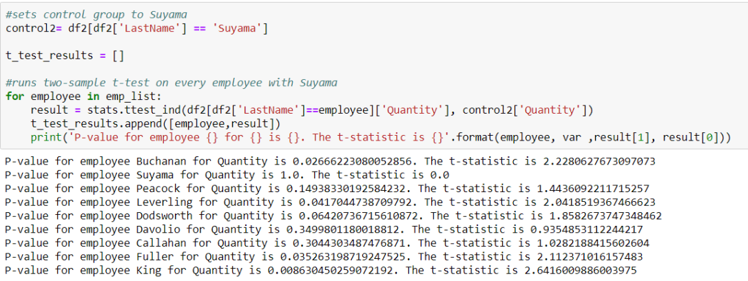
The results above for question #2 show that Buchanan, Leverling, Fuller, and King having significantly more sales quantity than Suyama. To check this, I also ran ANOVA and found similar results:

For question #3, the steps were almost identical to question #2, but I instead found an interesting contradiction. With t-test, none of my results were significant, so I presumed that no category of item sold more or less than other categories.

Yet, conducting ANOVA bore some different results.

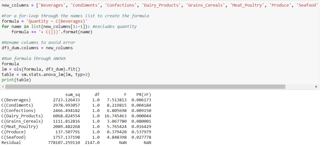
It seemed that beverages, condiments, confection, dairy, and seafood all had a significant impact on the items sold.  Even though these effects could not be detected with a student t-test, ANOVA is able to gauge the influences of each group collectively. With a bit more research, it would be interesting to see how different categories may spike according to different seasons or months. One would imagine that poultry sales would spike during the months of November and December.

For question #4, I wanted to do something with time series data, since I recently learned how to play with the data type. Although I couldn’t find anything about deliver date, I noticed that the there was an OrderDate and ShippedDate on the Product table, so I decided to query that information along with company names. Luckily for me, I only had three companies to work with.

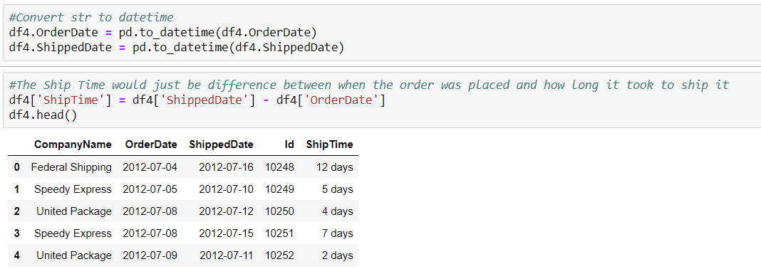
I noticed that both columns were strings, unlike what was written in the schema. I converted both OrderDate and ShippedDate to datetime, subtracted the OrderDate from the ShippedDate, and created a new column for the number of days it took called Shiptime.

From here, the process was almost exactly similar to questions 2 & 3. I constructed a null and alternative hypothesis, tested with an arbitrary control, revised, and then conducted an ANOVA test. This time, my t-test concurred with the results of the ANOVA.

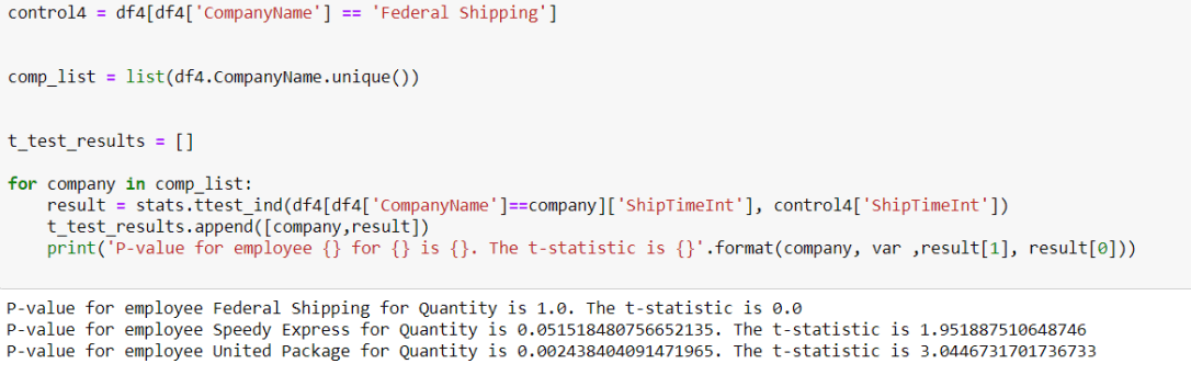
All shipping companies had an impact on the ship time, and United Package had the biggest impact. One important thing to note though is that in this case, having the biggest impact on the target variable is a negative outcome. Therefore, the best shipping company is Federal Shipping, since it had the lowest ship time.

Of course, fastest shipment does not always justify the costs, so further investigations would look into the cost of using one company over the other. After all, if every company delivered the items by the required date, then it may not be justifiable to use the faster company at a higher cost.

Overall, the Northwind Database gives a plethora of options for data exploration and analysis. It is not massive enough to be overwhelming nor is it too small to be a challenge.

 

¹ For those without a strong mathematics background or just need a refresher, the null hypothesis is the basic assumption that what you’re trying to find with the investigation is not true. If the results are not statistically significant enough, the null hypothesis must be accepted. This simply means that any differences found may be due to chance instead of any real effect.